Document Actions
gvSIG-Desktop 1.10. User Manual
- Geoprocessing tools
Geoprocessing tools
Introduction
The gvSIG geoprocessing extension allows you to apply a series of standard processes to the vector information layers loaded in the layer tree in a gvSIG view (ToC), thus creating new vector information layers which will provide new information for the source layers.
The following geoprocesses have been implemented in the first version of the geoprocessing extension:
- Buffer.
- Clip.
- Dissolve (by adjacents and alphanumerical criteria).
- Merge
- Intersection.
- Join.
- Spatial Join.
- Convex Hull (minimum convex polygon).
- Difference.
The output layer can take one of the output formats supported by gvSIG (it can only be saved in shp format at the moment).
When some geoprocessing tools are applied (for example, Clip) a window appears in which a spatial index can be created for the input layer. This is an internal process which is only carried out once per layer and per new project and speeds up the spatial intersection processes.

To create a spatial index for the input layer which can be used by the geoprocesses, click on “Yes”.
Accessing the geoprocesses
You can run the geoprocesses available in gvSIG with the geoprocessing wizard by clicking on the following tool bar button:

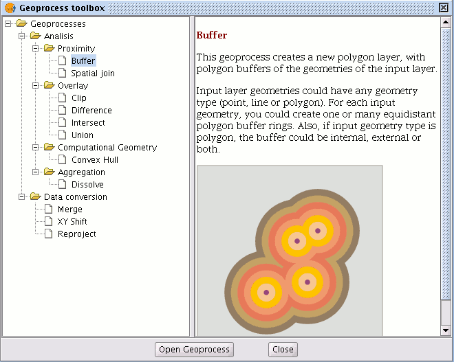
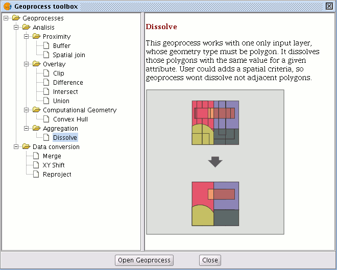
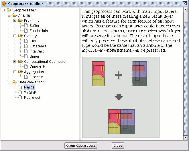
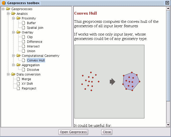
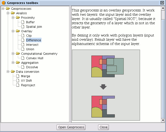
The “Geoprocess toolbox” will appear and you can use it to select the geoprocess you require. To access the different geoprocesses, pull down the tree in the window shown below (double click with the left button of the mouse on the "Geoprocesses" folder and the rest of the folders will appear).

When you have found the geoprocess you wish to use, click on the “Open geoprocess” button.

Buffer
Introduction
This geoprocess generates “areas of influence” around the vector element geometries (points, lines and polygons) of an “input layer”, thus creating a new polygon vector layer.
Several equidistant concentric radial rings can be generated around the input geometries. Moreover, in the case of polygon input geometries, the area of influence can be outside the polygon, inside the polygon or both inside and outside it. Some examples of the creation of areas of influence include:
- Which urban areas lack schools in a 1000m radius.
- Which wells do not comply with regulations on observing the minimum distance between two consecutive wells.
- River bed flood zones to monitor flood risks.
Creating an area of influence or buffer
When you click on the “Geoprocessing wizard” button, the following dialogue appears:
If you select “Buffer” and click on the “Open geoprocess” button, the window associated with this process is shown:
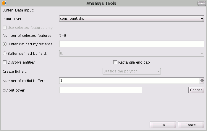
The form is divided into the following parts:

Selecting the elements whose buffer is to be computed. This is a pull-down list in which you can select the vector layer the calculation is to be applied to. If you wish, you can enable the “Use selected features only” check box so that the process only computes the buffer of the elements currently selected in the specified layer.
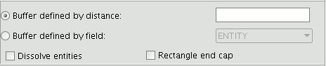
Inputting the features of the buffer to be computed. You can choose to input the buffer defined by distance (in the first text box) or to input a field in the input layer, from which the buffer radius value to be applied will be taken. This second option allows you to apply different buffer radii to different vector elements (whilst the first option applies the same radius to all the elements in the input layer). When the buffer of all the input layer elements has been generated, the “Dissolve features” option allows you to merge the elements whose geometries touch each other in a second iteration.
The “Rectangle end cap" option allows you to generate buffers with perpendicular edges (not rounded). Selecting the number of concentric buffers and their situation regarding the original geometry. The gvSIG “Buffer” geoprocess allows you to generate several equidistant areas of influence of the original geometry (for example, if the buffer distance to be applied is 200m and you choose to generate two concentric radial rings, the buffer distance of the second ring will be between 200-400m. Currently, you can only generate a maximum of three concentric radial buffer rings for efficiency reasons. If the vector layer we are working on is a polygon layer, the “Create Buffer…” option will be enabled, thus allowing the user to generate buffers outside, inside and both inside and outside the original polygon.

Introducing the result layer characteristics. Currently, the result of running a geoprocess can only be saved as an shp file. Thus, gvSIG allows you to select an existing shp file to overwrite it or to specify a new one. As new formats are supported to save the result of the geoprocesses, wizards will be provided to indicate the characteristics of these formats.

When you have input all the necessary information to compute the buffer, and clicked on the “Ok” button, a check routine is carried out to ensure that the information input is correct: whether the radius distance is numerical, whether the attribute from which the buffer radii are taken are numerical, whether a result file has been input, etc. If the check routine is not correct, a dialogue box appears so that the input data can be corrected.
If the input information that you have entered is correct, a window with a progress bar appears, in which the buffer processing rate is shown.
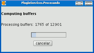
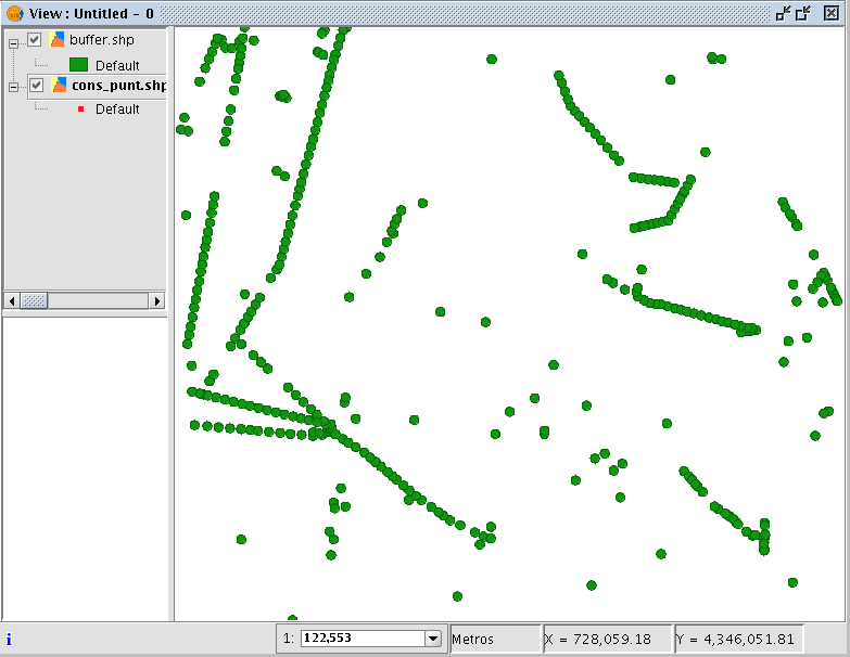
The process can be cancelled at any time by clicking on the “Cancel” button. As a consequence, the result file and any other intermediate product generated as a result of running the process are deleted. Whilst the buffer computing process is underway, other tasks can be carried out, such as changing the zoom or adding new layers to the layer tree in the gvSIG view. Other tasks can be carried out because all the geoprocessing extension geoprocesses are run in the background. When the process has finished, the new result layer is added to the layer tree in the active view. It is made up of buffer polygons with a specified radius based on the source layer.
Finally, the “Dissolve elements” option can be useful in specific situations (such as when the aim of computing the buffer polygons is to determine the total surface area affected by a phenomenon: quarantine areas, etc.), because when the generated polygons are merged the surface area covered by the buffer will be a real surface area, i.e. the sum of two buffers will not have any overlays.
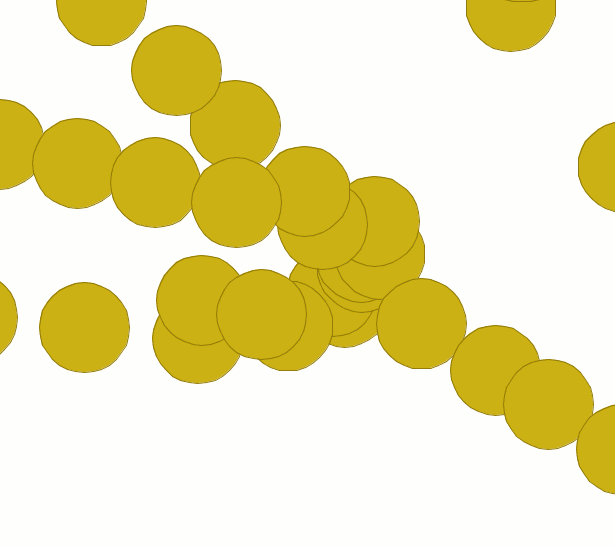
The above image shows non-merged overlay polygons. The total area covered by the phenomenon does not coincide with the sum of the individual areas.
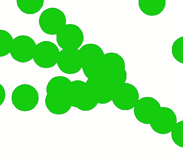
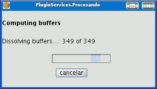
However, this second image shows merged overlay polygons. The total area covered by the phenomenon is real. When the buffer computing process includes the merger of overlay areas (dissolve) we cannot predict its exact duration (we do not know how many polygons will touch each other a priori). This is why the gvSIG geoprocessing extension does not show us a progress bar as such, it shows us a bar which periodically reaches the end and then goes back to the beginning. This type of process is called an “indeterminate” process.
Intersection
Introduction
This geoprocess operates on two layers, the “input layer” and the “overlay layer”, whose geometries can be polygons, lines or points.
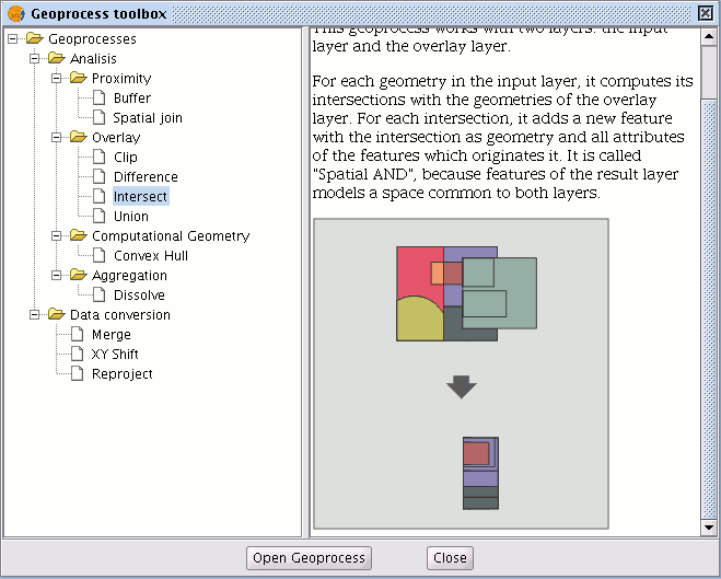
It calculates the intersection with the different geometries in the “overlay layer” for each geometry in the “input layer”, thus creating a new element for each intersection. This element will take all the alphanumerical attributes in the geometries that created it (input and overlay). This is why (it models space areas which comply with the condition of belonging to the two polygons, lines or points that created it) this geoprocess is known as “Spatial AND" operator.
An example of how this geoprocess can be applied:
Given a land use layer (e.g. Corine2000), and a national geological map layer, you can obtain a polygon layer with homogeneous information on land use and geological material.
Running the 'Intersection' geoprocess
After selecting the "Intersection" geoprocess, the following dialogue appears:
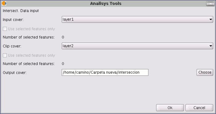
Select the input layer and the overlay layer. You must also specify a file in which to save the results. Finally, click on "Ok" and the geoprocess will be run.
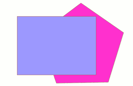
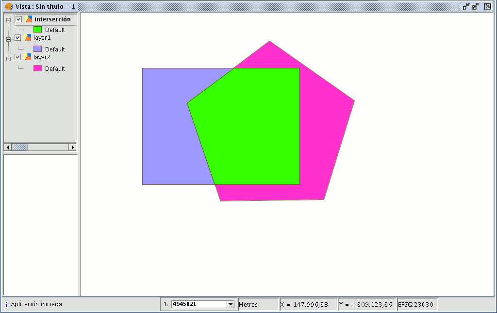
In this case, we will use a very simple example to better understand the function of the geoprocess. The previous figure shows two overlaying polygons. The result of launching the “Intersection” geoprocess with these layers as parameters is as follows:
Clipping
Introduction
This geoprocess allows you to limit the working area of a vector layer (points, lines or polygons), and to extract an area of interest from it.
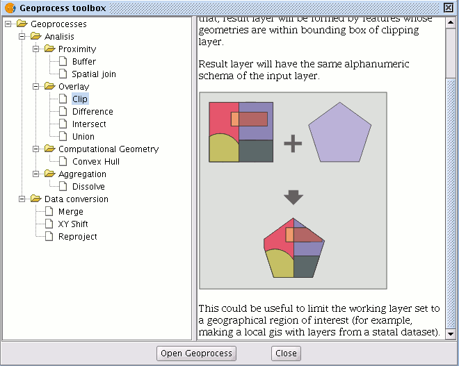
To do so, you need an “input layer” (the layer you will use to extract an area) and a “clipping layer” so that the union of the geometries included in the "clipping layer" defines the working area.
The geoprocess checks all the vector elements in the “input layer” and will calculate the intersections for the vector elements contained in the working area defined by the “clipping layer”, so that in the "result layer" only the vector elements of our working area will appear. The geometry portion that lies outside the working area will be clipped. The alphanumeric schema of the input layer remains intact.
Examples of use:
Setting up a local GIS would allow you to include national or regional maps and then to delimit the city or town as the working area.
Running the Clipping geoprocess
When the "Clip" geoprocess has been selected, the following dialogue appears.
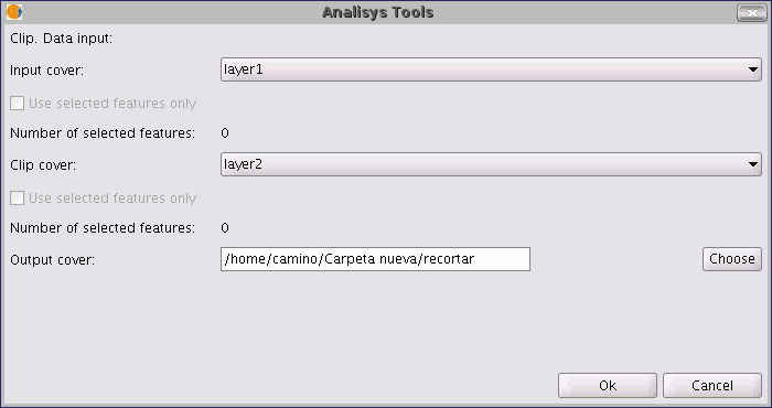
This dialogue allows you to select which layer you wish to clip, and gives you the chance to only clip the elements which are selected in the layer.
It allows you to select which layer will be used as the clipping layer and whether you wish to use the union of all the polygons in the clipping layer as the clipping polygon or just the selected elements.
Finally, as in the case of the other geoprocesses in gvSIG's geoprocessing extension, you can define how the result layer will be saved (at present you can only save it as a shp file).
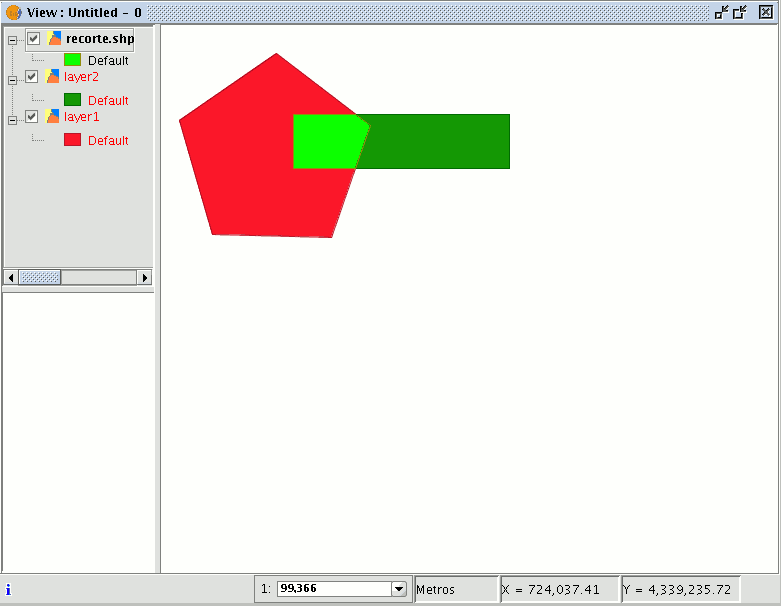
As a result of running the geoprocess, you will have a new layer in which only the geometries which came under the union of the clipping geometries have been kept.
Dissolve
Disolve
This geoprocess only acts on one “input layer”. The process analyses each entity in the "input layer" and merges the elements that have an identical value for a specific field into one element. Moreover, it allows you to involve spatial criteria in the decision to merge several features. This allows you to establish that for two elements to be merged, they must be adjacent to each other in addition to having the same value in the specified attribute.
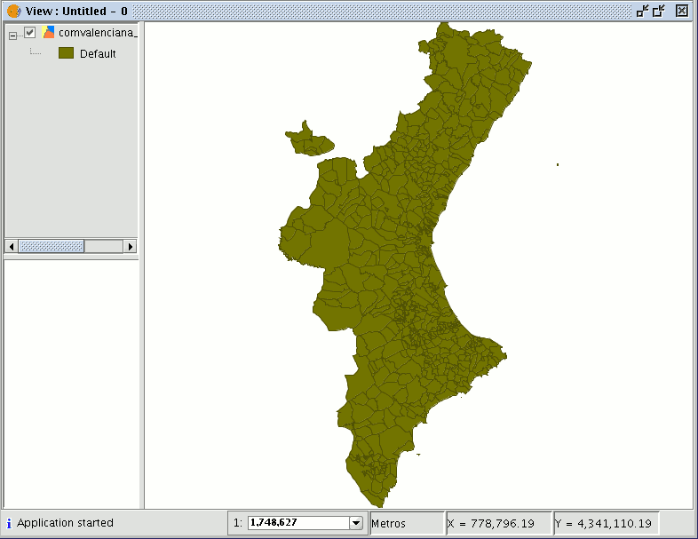
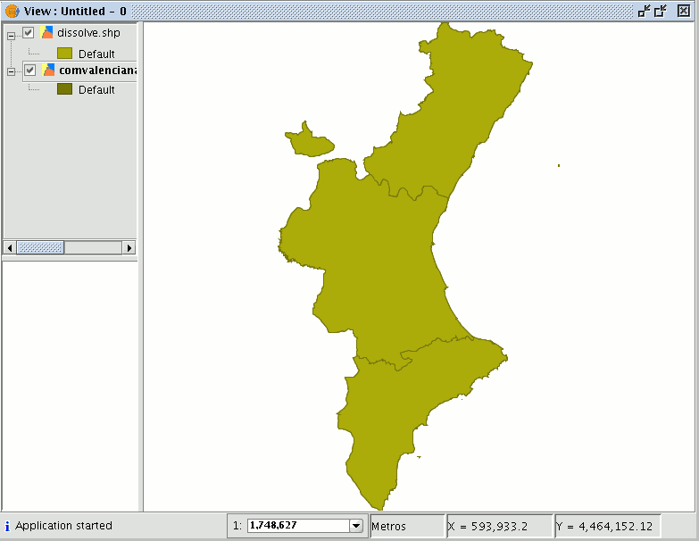
Example: We have a polygon layer which represents the municipalities of a particular autonomous region and we need a polygon layer with the provinces which make up this region. We can generate a province layer by launching the “Dissolve” geoprocess and specifying that the polygons that have the same value for the "PROV" field in which a unique code for the province is specified are merged.
Running the 'Dissolve' geoprocess
Using the previous example, we start by taking a "local layer" which we wish to convert into a "provincial layer".
When the "Dissolve" geoprocess has been selected, the following window appears:
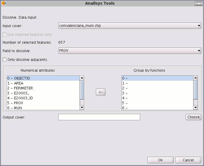
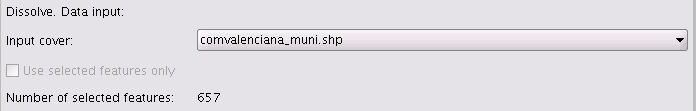
Firstly, select the layer you wish to dissolve (you can only work with a selection of elements in this layer).
You then need to specify the attribute of this layer which is going to be used as the criterion to merge the adjacent polygons. In our example, we must choose the “PROV” attribute.
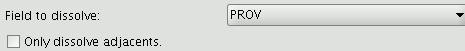
The polygons to be merged must have the same value for the dissolving attribute and in addition, you can choose whether they are adjacent to each other (spatial criteria). If you wish to choose this option, enable the "Only dissolve adjacents" check box. The gvSIG geoprocessing module allows you to keep a summary of the input layer polygon attributes once they have been merged. To do so, the “Summary function” concept is introduced. As each polygon of the “Dissolve” geoprocess result layer is the product of joining several input layer polygons, a summary function on the numerical attributes of the merged polygons can be applied.
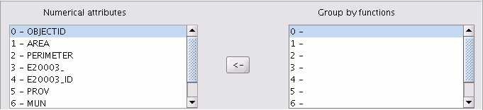
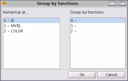
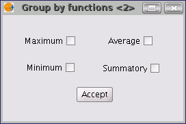
If you click on the button with the "<-" icon, a dialogue will be shown in which you can choose one of several summary functions for a selected attribute.
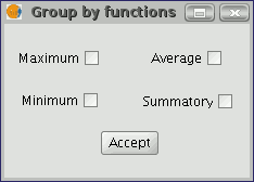
The summary functions supported are maximum, minimum, average and summatory. A field will be included in the result layer for each summary function selected for the numerical attributes you have selected a summary function for.
When you have specified the field you wish to merge and the numerical attributes you wish to obtain a summary value for in the result layer, you are ready to run the geoprocess.
Merge
Introduction
This geoprocess acts on one or several layers, generating a new layer which joins all the geometries in the “input layer”. The "result layer" of this geoprocess will keep the attributes of the "input layer" specified by the user. For the rest of the layers which have not been selected, the attributes whose name and type of data coincide with any of the attributes in the selected layer will be kept.
Example:
When a cartographic series arrives which is separated into sheets and you wish to join the content of the different sheets in one layer. This is the case of the Magna series of sheets, published by the Spanish Technological and Geomining Institute (ITGME).
Running the 'Merge' geoprocess
If you select the “Merge” geoprocess, the following dialogue appears:
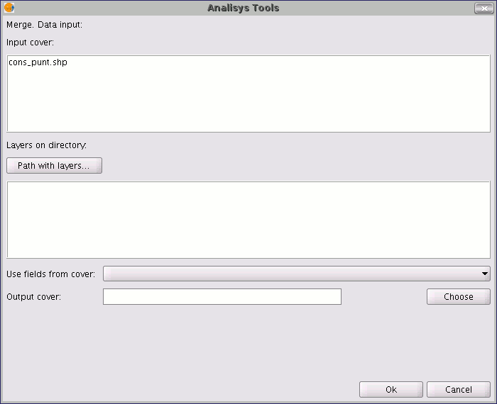
The geoprocess allows any of the layers loaded in the layer tree in the gvSIG active view as an input layer. To run the process, first select the layers you wish to merge in the "Input layers" text box. Then, click on the "Select” button. A new window will open in which you can give the new layer file a name or choose a target file.
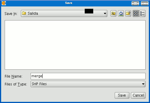
Click on the "Save" button when you have finished and gvSIG will return you to the geoprocess window. Click on the "Ok" button. This will start the geoprocess.
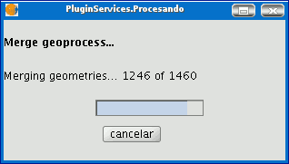
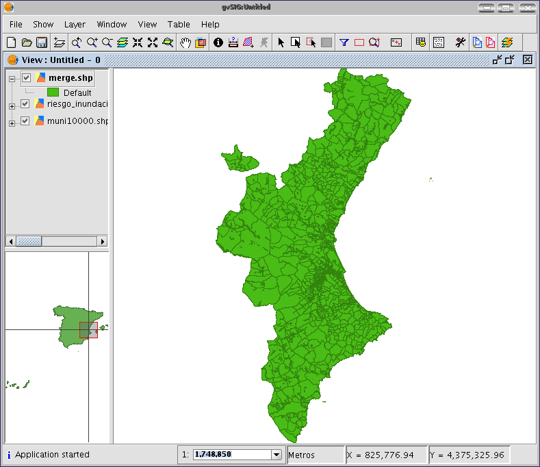
A new layer will be created at the end of the process which will be added to the view.
However, in the example of the sheets in a cartographic series, it would be awkward to load all the pages in the series one by one. Thus, there is an extra option to select a directory and to add all the layer files (with extensions supported by gvSIG) contained in this directory to the geoprocess input layer list. The only layer files currently supported are shp format files. If you click on the “Folder with files...” button and select a directory, a list of the layer files contained in it are shown and can be selected as part of the geoprocess input layers.
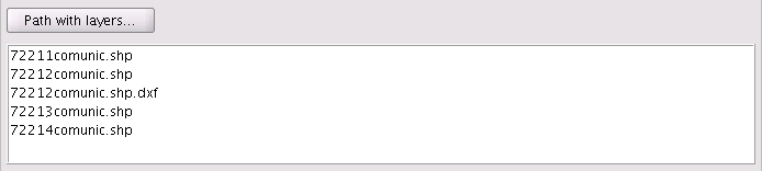
Until you select at least one layer to merge with one of the two possible lists (the layer list in the gvSIG layer tree and the layer list contained in the specified directory), no layer will be shown in the pull-down list. This list allows you to select which layer is going to define the attributes of the result layer’s attributes. When you select the layers to merge in one of the two lists, the layer whose attributes we wish the result layer to have and when you have specified the file you wish to save the result layer in, you can run the geoprocess. An initial requirement is that all the geoprocess input layers have the same type of geometries.
The result will be a new layer with all the input layer geometries.
Convex hull
Introduction
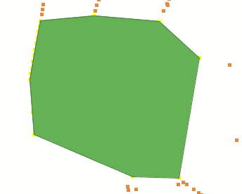
This geoprocess calculates the “Convex hull”, or the smallest convex polygon which surrounds all the vector elements in an “input layer”.
It only works with an “input layer” whose geometry type can be any type (point, line or polygon). There are different types of applications for this geoprocess: Determining the coverage area for a specific geographical phenomenon.
Calculating the diameter of the area covered by a series of geometries, etc.
Creating a convex hull
If you select the “Convex hull” geoprocess, the following dialogue appears:
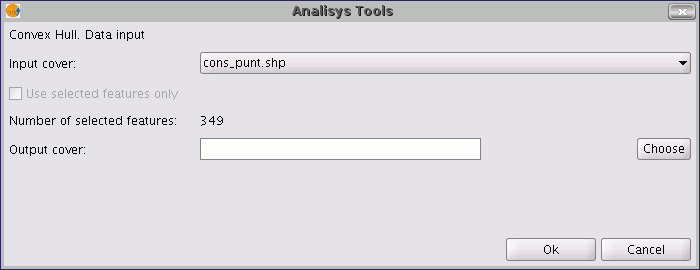
After selecting the layer whose “Convex Hull” you wish to calculate and specifying an shp result file, you can run the geoprocess and generate a new result layer.
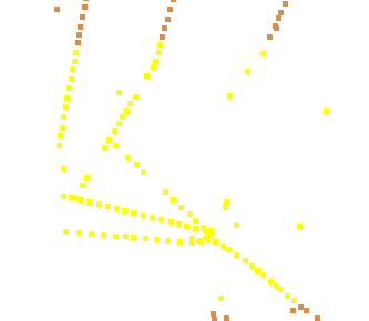
The following image shows the convex hull created which surrounds all the points in the input layer.
Difference
Introduction
The “Difference” geoprocess works with two layers, the “input layer” and the “overlay layer”. It is known as “Spatial NOT” and allows you to obtain the areas in a layer which are not present in the other layer. The geometries in both the “input layer” and the “overlay layer" must be polygons, lines or points. The alphanumerical schema of the “input layer” will remain intact in the "result layer", as in the end it gives more information about it.
This geoprocess is very useful in numerous situations. For example, it can be used to complement the "Clip" geoprocess. If “Clip” allows you to exclude everything that does not belong to a geographical area under study, "Difference" allows you to do exactly the opposite; exclude a specific area from our working layer.
A useful example:
Transferring territorial jurisdiction between different governing bodies. Thus, if the national government transfers certain jurisdiction to a regional authority, it can decide to exclude the geographical area of the transfer in question from its data bases.
Running the 'Difference' geoprocess
Running the “Difference” geoprocessClick on the “Open Geoprocess” button to access the dialogue window which allows you to run the "Difference" geoprocess.
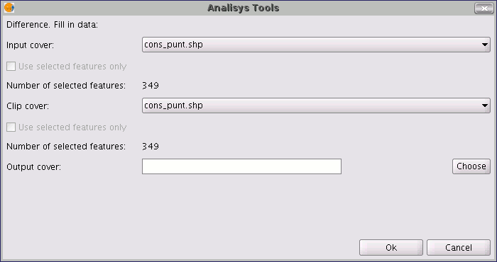
You can enable the “selected features” check boxes at this point of the geoprocess for the input layer and the overlay layer. If you click on the “Ok” button, the geoprocess will be run.
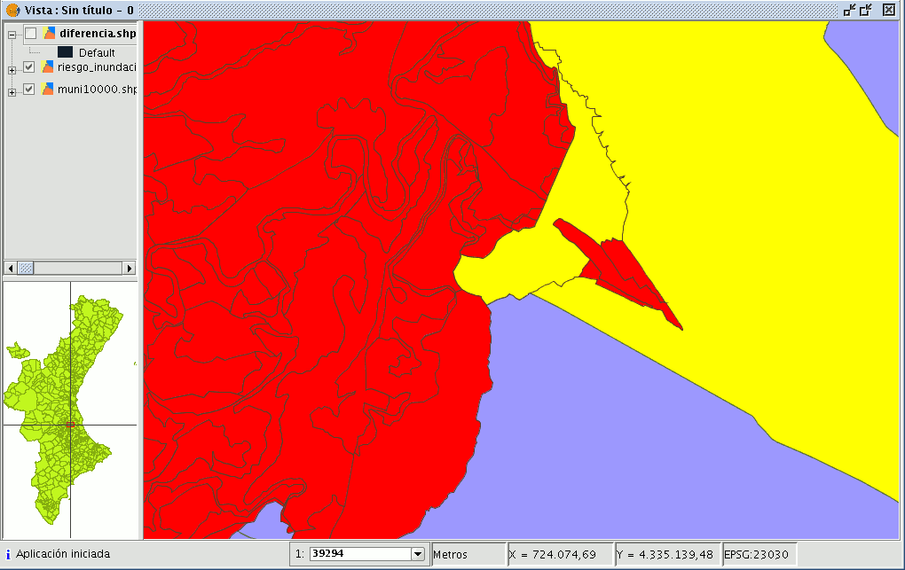
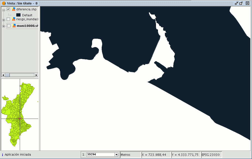
In the following image, the “Difference” geometry appears in black between a flood zone and one of the selected cities or towns. In this case, the new layer resulting from the calculation of the difference will take the schema (alphanumerical attributes) of the geoprocess input layer.
Union
Introduction
This geoprocess is similar to the “Intersection” and "Difference" geoprocesses in that it operates on two polygon, line or point layers to obtain their intersections (this is why these three geoprocesses are known as “overlay geoprocesses”).
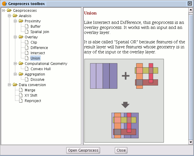
The "Union" geoprocess is known as "Spatial OR", because the result layer is made up of the geometries which appear in the two layers (intersections between the polygons, lines or points), plus the geometries which only appear in one of the two associated layers.
This means that the geoprocess carries out three analyses:
the first time it calculates the intersection of both layers, the second time it calculates differences between the first layer and the second, and the third time it calculates the differences between the second layer and the first.
This geoprocess may be of interest if you wish to generate new layers which show the occurrence of two phenomena so that the occurrence of one of the two or of both is highlighted.
Running the "Union" geoprocess
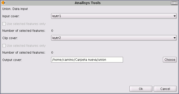
If you select the “Union” option, the following dialogue appears:

When you have selected the input layer, the clip layer and an output layer, click on "Ok".
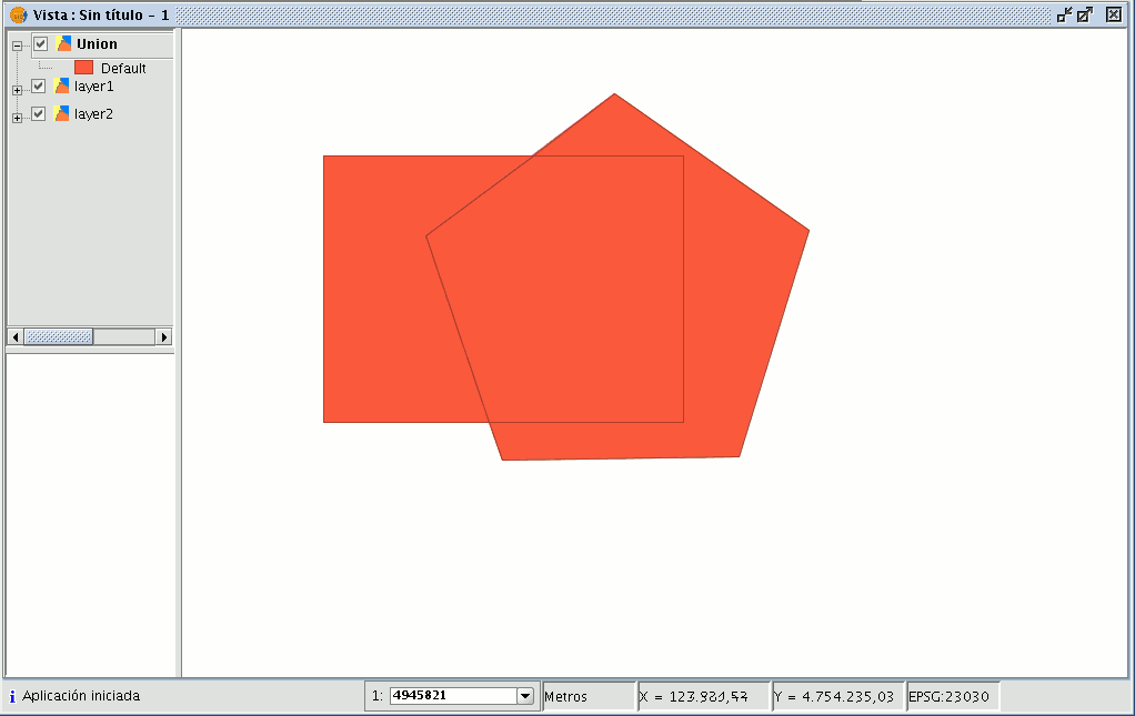
The result layer will have all the intersections and differences between the two layers. If you click on the “Information” button and then on the different polygons in the result layer, you will see that the intersections have all the attributes, whilst the differences only have the attributes of the layer that created them.
Spatial join
Introduction
This geoprocess allows you to transfer the attributes of one layer to another based on a common element. In contrast to the join sql operator in the relational data bases, in this case, the common element is not that a field of the two tables takes the same value, but that the related elements in the two layers meet some spatial criteria.
The “Spatial join” geoprocess allows you to follow two types of spatial criteria to establish the spatial link:
Nearest neighbour (1->1 relationship). This assigns the attributes of the nearest element in the related layer to an element in the source layer.
If the nearest element intersects (or in the case of polygons is “Contained in”) with the source element, the algorithm will take the first element analysed in the possible intersections.
Contained in (1->M relationship). This relates an element in the source layer with several elements in the destination layer (in particular, with those that intersect).
In this case, the source layer will not inherit the related layer’s attributes, but the operation will be very similar to the "Dissolve" geoprocess.
The user can choose one or several summary functions (average, minimum, maximum, summatory) to be applied on the numerical attributes of the related layer for the M elements related to an element in the source layer.
Running a 'Spatial Join'
When you have selected the "Spatial join" option, the following window appears:
This window is practically the same as the windows in the overlay geoprocesses (Union, Difference, Intersection) with one difference.
It allows you to choose whether you want to run a 1-1 relationship (using the nearest neighbour spatial criterion) or run a 1-N relationship (using the “Intersect” or “Contained in” spatial criterion).
The choice can be made by enabling or disabling the "Use nearest geometry" check box. If when you have selected the source layer and the layer to be related, the geoprocess is launched and you have not enabled the "Use nearest geometry" check box, a window appears in which you can select the summary functions you wish to apply for each numerical attribute of the layer to be related:
The summary functions are the same as in the “Dissolve” geoprocess:
Thus, the attributes transferred to the source layer will be the result of the summary functions selected for each numerical field. If you run the geoprocess and the “Use nearest geometry” option is enabled, this window does not appear.
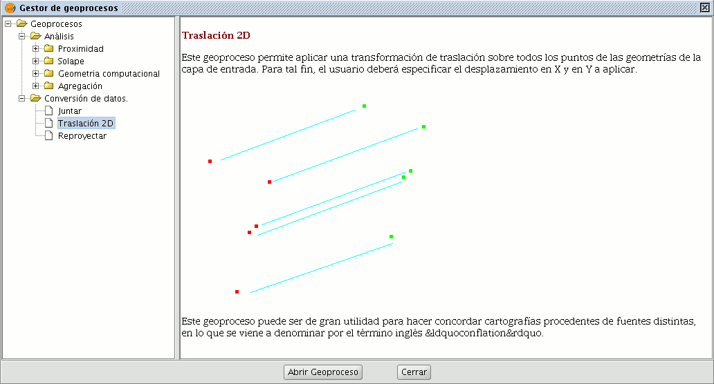
2D Translation
Introduction
This geoprocess allows a translation transformation to be applied to all the points, lines and polygons of the geometries in the input layer. The geoprocess can be applied to all types of vector layers (shp, dgn, dxf…). To do so, the movement on X and Y must be specified.
This geoprocess is extremely useful when combining cartographies which come from different sources, a process which is referred to as conflation. Bear in mind that although translations can be carried out on all types of vector layers (shp, dgn, dxf, dwg…), the resulting output layer will always be a shape file. In other words, the input layer can be a shp, dxf or dgn file, but when translation is applied to these layers, the result will be one or various different output layers which are always shape files.
When a translation is carried out in which the input layer is a vector layer which is not a shape file, the result of the translation will be three layers in SHP format (one line layer, one point layer and one polygon layer).
If, for example, the input layer to which the translation is applied contains only points and lines, the polygon .shp file will be created but it will be empty.
NB. At the end of this section there is a table giving details of the relationship between the type of input file and the resulting output layer.
Translating a vector layer
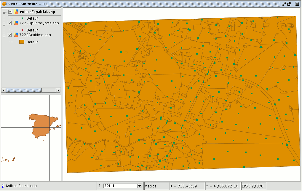
Firstly, load a vector layer in gvSIG and then click on the geoprocessing wizard in the tool bar.

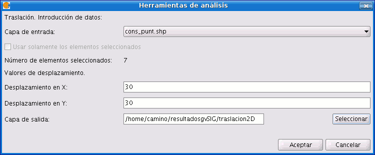
Select the option “2D Translation” from the “Data Conversion” folder. Click on the “Open Geoprocess” button and the geoprocess data input window opens. For the input layer, select the vector layer (dgn, dxf, dwg, shp…) you wish to translate and introduce the values corresponding to X and Y. Select an output layer and click on “Ok”.
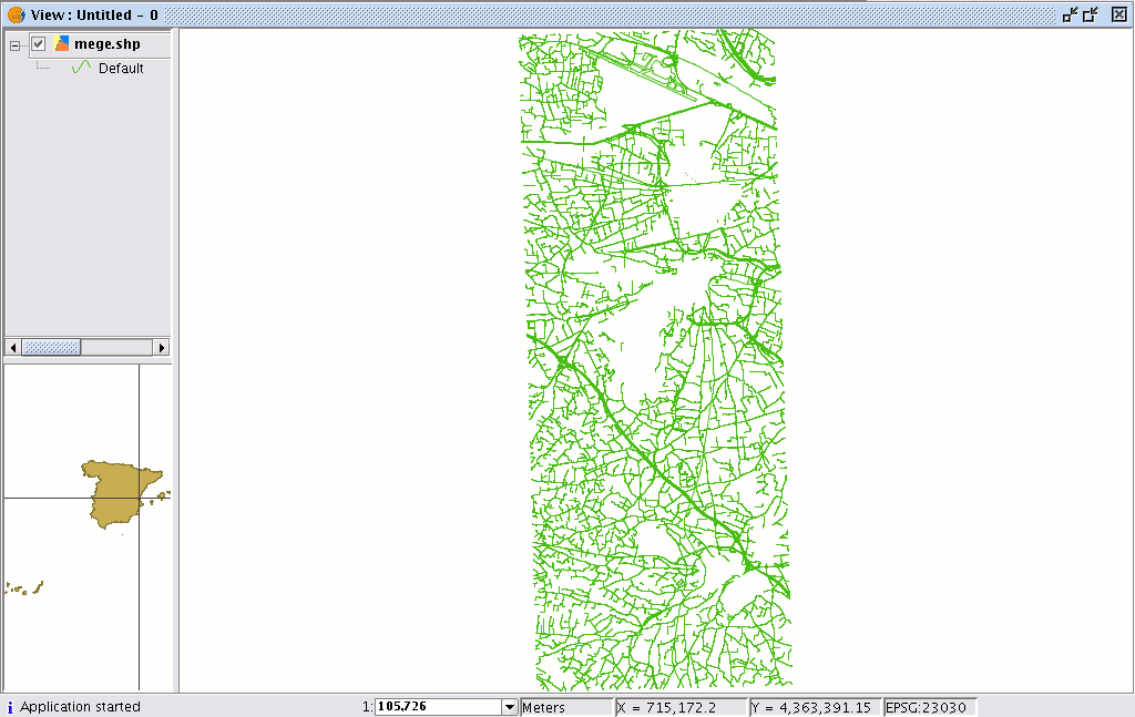
The following image shows the result of applying the translation process.
Relationship between the type of layer before and after translation.
| Input cover | Output cover/s | |
|---|---|---|
| Point Shp file | Point Shp file | |
| Multipoint Shp file | Multipoint Shp file | |
| Line Shp file | Line Shp file | |
| Polygon Shp file | Polygon Shp file | |
| Dxf (points, lines, polygons) | Point Shp file Line Shp file Polygon Shp file |
|
| Dgn (points, lines, polygons) | Point Shp file Line Shp file Polygon Shp file |
|
| Dwg (points, lines, polygons) | Point Shp file Line Shp file Polygon Shp file |
|
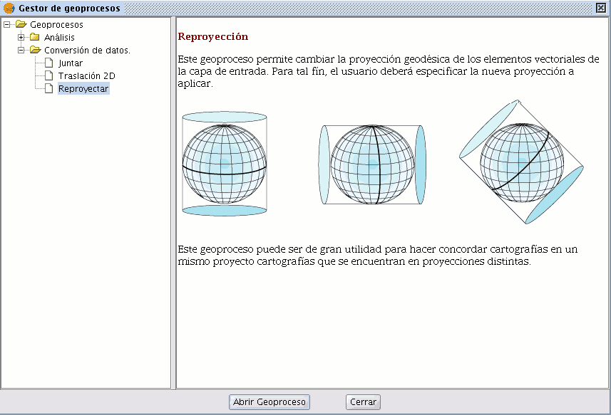
Reprojection
Introduction
This geoprocess allows you to change the geodesic projection of the vector elements in the input layer. In order to do so, the user must specify the new projection to be applied.
This process is extremely useful when standardising cartographies in the same project if these are in different projections.
Reprojection of a layer
Click on the geoprocessing wizard in the tool bar and select the “Reproject” option from the “Data conversion” folder.
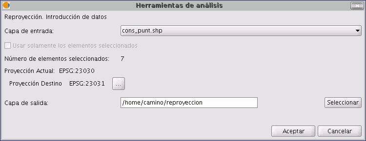
Click on “Open geoprocess”. The wizard will open to guide you through the reprojection process.
In “Input layer”, select the layer you wish to reproject from the layers loaded in the ToC.
To select the new projection for the layer, click on the button next to the destination projection and select the new reference system.